Imagine a detective standing in front of a map covered in red pins. Each pin marks a crime scene from a serial offender. The question isn't just where the crimes happened, but where the person committing them sleeps. This is the core promise of geographic profiling, a criminal investigative methodology that uses the locations of connected crimes to estimate an offender's most probable home or base of operations. It turns chaos into data, helping police narrow down thousands of suspects to a handful of likely neighborhoods.
Unlike general crime mapping, which looks at broad trends like "burglaries are up in District 4," geographic profiling is intensely personal. It asks, "Where does *this specific* offender live?" By analyzing the spatial patterns of incidents such as serial murder, rape, arson, or robbery, investigators can create a probability surface-a heatmap-that highlights small areas where the culprit is statistically most likely to reside. This method saves time, money, and resources by focusing door-to-door canvassing and surveillance on high-yield zones rather than spraying efforts across an entire city.
The Theory Behind the Map
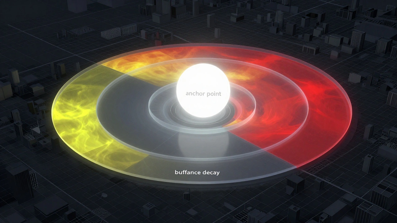
Geographic profiling isn't magic; it’s built on solid criminological theories developed over decades. At its heart lies the concept of the anchor point. Most offenders operate from a familiar base-usually their home, workplace, or a regular hangout spot. They don’t pick random locations for their crimes out of thin air. Instead, they travel from this anchor point through their daily routines.
This leads to two critical principles: distance decay and the buffer zone. Distance decay means that the likelihood of an offender committing a crime decreases as the distance from their anchor point increases. People generally prefer convenience and familiarity. However, there’s a twist. Most criminals avoid offending right next door to their house because the risk of being recognized by neighbors is too high. This creates a buffer zone-a ring around the home where crime probability is low. The danger rises slightly beyond this buffer before eventually decaying again as distance grows.
These behaviors are rooted in routine activity theory, which suggests crime happens when a motivated offender, a suitable target, and a lack of guardianship converge in space and time. Geographic profiling maps these convergences. It assumes offenders have cognitive maps of their surroundings and make rational trade-offs between effort, risk, and reward. If you understand how someone moves through space, you can predict where they start their journey.
How Investigators Build a Geoprofile
Creating a geoprofile is a structured process that blends qualitative insight with quantitative analysis. It doesn’t happen overnight, and it requires careful preparation.
- Case Linkage: The first step is ensuring the crimes are actually connected. Analysts must confirm that a series of incidents-say, five sexual assaults or three arsons-share enough similarities in modus operandi and timing to be attributed to one offender. If the crimes aren’t linked, the profile will fail.
- Data Collection: Precise geographic coordinates for each crime location are gathered. This includes offense sites, abduction points, and body disposal sites. These addresses are geocoded and imported into Geographic Information Systems (GIS).
- Model Specification: Analysts set parameters based on the case details. They define the minimum and maximum distances from the anchor point, adjust the buffer zone size, and decide if certain incidents should weigh more heavily than others (e.g., a murder might carry more weight than an attempted assault).
- Computation: Software divides the study area into a raster grid of tens of thousands of cells. For each cell, it calculates a likelihood score indicating the probability that the offender’s anchor point is located there. This generates a color-coded probability map.
- Interpretation: Detectives focus on the highest-probability zones. These areas often represent only a few percent of the total search area but capture the highest concentration of expected offender locations.
- Refinement: As new crimes occur or new evidence emerges, the model is updated. The geoprofile evolves, becoming sharper and more accurate over time.
Tools and Algorithms: The Engine Room
You can’t do modern geographic profiling with just a pencil and paper. It relies on sophisticated algorithms and specialized software. The most widely recognized formal model is Criminal Geographic Targeting (CGT), developed by Canadian criminologist Kim Rossmo. His algorithm mathematically implements distance decay and buffer zones, evaluating every grid cell on the map against the pattern of crime sites.
Today, the dominant commercial tool implementing these concepts is Rigel, developed by Environmental Criminology Research Inc. (ECRI) in Canada. Rigel integrates Bayesian statistical analysis, allowing investigators to combine spatial data with other evidence sources optimally. For instance, if intelligence suggests the offender owns a car, the model can factor in road networks and driving times rather than just straight-line distances.
While exact pricing for Rigel isn’t publicly listed-it’s typically sold via quote-based contracts to law enforcement agencies-the investment is considered essential for major departments. The software runs alongside standard GIS platforms, overlaying crime locations with demographic data, landmarks, and infrastructure. This integration allows analysts to see not just where the offender likely lives, but what kind of environment suits their behavior.
When Does It Work Best?
Geographic profiling shines in cases involving multiple events linked to a single actor. It is most commonly applied to:
- Serial Murder and Rape: These are the classic use cases. With hundreds of tips and suspects, a geoprofile helps prioritize who to interview first.
- Arson and Bombing: Serial arsonists often return to familiar areas. Mapping fire scenes can reveal a pattern leading back to the source.
- Robbery and Terrorism: When a sequence of robberies or terrorist plots shares spatial characteristics, profiling can identify the operational base.
- Cold Cases and Homicides: Even in one-off murders, if there are clues about victim movement or body disposal, spatial analysis can suggest likely recovery zones or suspect residences.
However, it has limits. If an offender is highly mobile-like a long-distance truck driver or someone traveling specifically to commit crimes far from home-the assumptions of distance decay break down. In these cases, the buffer zone may disappear, and the profile becomes less reliable. Additionally, poor data quality, such as inaccurate address geocoding, can distort results significantly.
Geographic Profiling vs. Crime Mapping
It’s easy to confuse geographic profiling with general crime mapping, but they serve different masters. Crime mapping is place-centered. It answers questions like, "Where are burglaries concentrated in the city?" This helps allocate patrol resources broadly. Hotspot analysis identifies areas of high crime density for strategic planning.
Geographic profiling is offender-centered. It ignores general hotspots unless they relate to the specific suspect. A burglar might operate in a hotspot, but geographic profiling tries to find where that specific burglar sleeps. While crime mapping supports community safety and resource allocation, geographic profiling supports individual suspect identification and apprehension. One paints the background; the other zooms in on the subject.
| Feature | Crime Mapping / Hotspot Analysis | Geographic Profiling |
|---|---|---|
| Focus | Place-centered (where crime occurs) | Offender-centered (where offender lives) |
| Goal | Resource allocation, trend identification | Suspect prioritization, arrest support |
| Data Requirement | Aggregate crime statistics | Linked series of specific incidents |
| Key Theory | Broken windows, routine activity | Distance decay, buffer zone, anchor point |
| Output | Heatmaps of crime density | Probability surface of offender residence |

Pitfalls and Limitations
Despite its power, geographic profiling is not a crystal ball. It produces probabilities, not certainties. Investigators must guard against over-interpreting the results. Just because a neighborhood lights up on the map doesn’t mean the offender definitely lives there; it just means it’s the most likely option among many.
Another risk is confirmation bias. If detectives already have a suspect, they might tweak the model parameters to fit that suspect’s location, undermining the objectivity of the analysis. Proper training is crucial. Analysts need to understand environmental criminology well enough to know when the model’s assumptions are violated. For example, if a killer deliberately dumps bodies far away to confuse police, the standard distance-decay model may mislead.
Furthermore, geographic profiling should never stand alone. It works best when combined with traditional detective work, forensic evidence, and behavioral profiling. It narrows the field, but it doesn’t catch the criminal. You still need fingerprints, DNA, or witness statements to make an arrest.
The Future of Spatial Investigation
As technology advances, so does geographic profiling. We’re seeing deeper integration with real-time data sources, such as GPS traces from vehicles or mobile phones. Bayesian methods are becoming more sophisticated, allowing models to update dynamically as new information arrives. Training programs at institutions like Texas State University are institutionalizing these skills, moving GP from a niche innovation to a standard component of advanced crime analysis curricula.
We also see expansion into non-traditional areas. Concepts of anchor points and distance decay are being applied to wildlife poaching and epidemiological spread, treating illegal acts or disease transmission as spatially structured behaviors. This cross-pollination strengthens the underlying science, making criminal investigations even more precise.
What is the difference between geographic profiling and criminal profiling?
Criminal profiling (or psychological profiling) focuses on the offender's personality, motives, and behavioral traits to predict future actions. Geographic profiling focuses strictly on the spatial patterns of crimes to estimate where the offender lives or operates. They are complementary tools: one tells you who the person might be, the other tells you where to look for them.
How accurate is geographic profiling?
Accuracy depends heavily on data quality and case suitability. In ideal scenarios with a clear series of linked crimes and stable offender habits, it can narrow search areas to a few percent of the total jurisdiction. However, it provides probabilities, not guarantees. It is most effective when used to prioritize suspects rather than pinpoint a single address.
Can geographic profiling be used for single-crime cases?
Traditionally, no. Geographic profiling requires a series of linked incidents to establish a spatial pattern. However, recent applications have extended to one-off murders or cold cases by analyzing limited spatial clues, such as victim routes or body disposal sites, to infer likely anchor points or search bases.
What software is used for geographic profiling?
The most prominent commercial software is Rigel, developed by ECRI. It uses Bayesian statistical analysis and integrates with GIS platforms. Other tools exist, but Rigel is widely cited in academic and operational contexts for implementing Rossmo’s Criminal Geographic Targeting algorithm.
Why do criminals have a buffer zone?
A buffer zone exists because most offenders want to avoid recognition. Committing a crime immediately next to their home increases the risk of being seen by neighbors or family. Therefore, they travel a short distance away from their anchor point before offending, creating a low-probability ring around their residence.