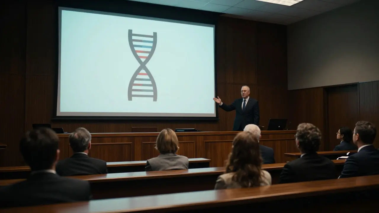
Imagine a jury hearing that the DNA found at a crime scene matches the suspect. The prosecutor says, "The odds of this being a coincidence are one in a billion." Does that mean the suspect is guilty? Not necessarily. That number is a DNA population genetics calculation, specifically a probability statement about how common a specific genetic profile is in a given group of people. It tells you how rare the evidence is, not who left it there.
This distinction trips up even seasoned legal professionals. To understand what those numbers actually mean, we have to look under the hood of forensic DNA analysis. We need to see how scientists count genes in populations and apply statistical laws to predict how likely it is for an unrelated person to share the same genetic markers.
The Core Concept: What Is Population Genetics?
Population genetics is the study of genetic variation within groups of organisms, focusing on how gene frequencies change over time and across different subgroups. In the context of forensics, we aren't interested in evolution or natural selection. We care about one specific thing: the baseline frequency of certain DNA variants in a relevant population.
When a lab analyzes a DNA sample, they look at specific regions called Short Tandem Repeats (STRs). These are non-coding sections of DNA where short sequences repeat. The number of repeats varies from person to person. For example, one person might have 12 repeats at a specific locus, while another has 14. By looking at multiple loci-usually 20 or more in modern kits-we create a unique genetic fingerprint. But to say that fingerprint is "rare," we need to know how many other people in the world have that same combination.
This is where the data comes in. Laboratories maintain large databases of allele frequencies. An allele is a variant form of a gene. If I test 10,000 individuals from a specific geographic region and find that 5% of them carry a specific allele at Locus D8S1179, then the frequency of that allele is 0.05. This baseline data allows us to calculate the likelihood of finding that pattern by chance.
How Probabilities Are Calculated: The Math Behind the Match
You don't just guess these numbers. They are derived using specific statistical models. The most fundamental rule here is the Hardy-Weinberg equilibrium is a principle stating that allele and genotype frequencies in a population will remain constant from generation to generation in the absence of other evolutionary influences. While human populations don't perfectly follow this ideal model due to migration and mating patterns, it provides a solid mathematical framework for estimating genotype frequencies from allele frequencies.
Let's break down the calculation for a single locus. Suppose the frequency of Allele A is 0.3 and the frequency of Allele B is 0.4. Under Hardy-Weinberg assumptions, the probability of someone having two copies of Allele A (homozygous) is $0.3 \times 0.3 = 0.09$. The probability of having one copy of each (heterozygous) is $2 \times 0.3 \times 0.4 = 0.24$. The factor of 2 accounts for the fact that you can inherit A from mom and B from dad, or vice versa.
In forensic cases, we usually deal with heterozygous profiles because they are more informative. Once we have the probability for one locus, we multiply the probabilities across all tested loci. This is known as the Product Rule. If you have 20 independent loci, and each has a low probability of matching, the combined probability becomes astronomically small. This is how we arrive at those "one in a trillion" figures often cited in courtrooms.
| Profile Type | Description | Typical Random Match Probability (RMP) | Evidentiary Value |
|---|---|---|---|
| Full Profile (20+ STRs) | All loci present and clear | < 1 in 10^15 | Very High |
| Partial Profile (10-15 STRs) | Some loci missing or degraded | 1 in 10^6 to 1 in 10^12 | Moderate to High |
| Mixed Sample | DNA from two or more contributors | Variable (requires complex modeling) | Depends on deconvolution accuracy |
| Y-STR / mtDNA | Uniparental inheritance | Higher (more common in population) | Lower (exclusionary power only) |

The Role of Subpopulations and Database Choice
Here is where it gets tricky. Humans are not a single, randomly mixing pool. We have subpopulations based on ancestry, geography, and ethnicity. If you use a database built entirely from European Americans to calculate the probability for a suspect of East Asian descent, your math might be off. Some alleles are more common in some groups than others.
To handle this, forensic labs use conservative estimates. Instead of picking the exact ethnic background of the suspect (which can be biased or inaccurate), they often use a "worst-case scenario" approach. They calculate the probability using the highest frequency observed across all major subpopulations in their reference database. This ensures that the reported probability is not overstated. If the true probability is lower, the evidence is stronger than stated. If it's higher, the worst-case estimate covers it.
Another critical concept is Allele Frequency is the proportion of a specific allele among all alleles at a particular locus in a population. These frequencies are not static. They change slowly over generations but can also shift due to recent migrations. Therefore, reference databases must be updated regularly. Using outdated frequency data can lead to inaccurate probability statements, potentially undermining the credibility of the entire case.
Random Match Probability vs. Likelihood Ratio
Many people confuse the Random Match Probability (RMP) with the Likelihood Ratio (LR). Let's clarify the difference because they serve different purposes in the courtroom.
The RMP answers the question: "If a random person were picked from the population, what is the chance they would have this DNA profile?" It is a simple frequency count. It does not account for the prosecution's hypothesis (the suspect did it) versus the defense's hypothesis (someone else did it). It is a measure of rarity.
The Likelihood Ratio is more sophisticated. It compares the probability of seeing the evidence if the suspect is the source versus the probability of seeing the evidence if an unknown person is the source. Formulaically, it is $P(Evidence | Suspect) / P(Evidence | Unknown)$. In many straightforward full-profile cases, the numerator is close to 1 (if the suspect is the source, the evidence should match), and the denominator is the RMP. So, the LR is roughly the inverse of the RMP. However, in mixed samples or partial profiles, the LR requires complex probabilistic genotyping software to account for stochastic effects like drop-in and drop-out. This makes the LR a more robust metric for complex cases, though the RMP remains easier for juries to grasp intuitively.
Pitfalls and Common Misinterpretations
Even with rigorous math, humans make mistakes. One common error is the Prosecutor's Fallacy. This occurs when the probability of the evidence given the defendant's innocence is confused with the probability of the defendant's innocence given the evidence. Just because the DNA match is rare doesn't mean the suspect is guilty beyond reasonable doubt. There could be innocent explanations: lab contamination, family members sharing similar profiles, or a coincidental match (though extremely unlikely with full profiles).
Another pitfall is ignoring population structure. If a suspect belongs to a small, isolated community, the effective population size is smaller than the national database suggests. This can increase the probability of related individuals sharing similar profiles. Forensic experts adjust for this using theta values ($\theta$), which correct for subpopulation clustering. Failing to apply these corrections can lead to overly optimistic probability statements.
Finally, consider the quality of the DNA itself. Degraded DNA leads to partial profiles. With fewer loci, the discriminative power drops significantly. A profile with only 8 loci might have a random match probability of 1 in 1 million, which is not nearly as compelling as 1 in a quadrillion. Jurors need to understand that "match" doesn't always mean "unique identifier." It means "consistent with," and the strength of that consistency depends heavily on the completeness of the data.
Practical Implications for Legal Professionals
For lawyers and judges, understanding these nuances is crucial. When cross-examining a forensic expert, ask about the reference database used. Was it local or national? How old is the data? Did they use the product rule correctly? Were any loci excluded due to poor quality, and how did that affect the final probability?
Also, pay attention to how the expert presents the numbers. Do they say "there is a 1 in a billion chance of a random match" or "the likelihood ratio is one billion to one"? The former is a frequency; the latter is a comparative weight of evidence. Both are valid, but they require different interpretations. Understanding the underlying DNA population genetics principles allows you to challenge flawed methodologies and ensure that the statistical evidence presented to the jury is both accurate and fairly represented.
Ultimately, DNA evidence is powerful, but it is not magic. It is a tool based on statistics and biology. By demystifying the probability statements, we empower everyone involved in the justice system to make better, more informed decisions.
What is the difference between a random match probability and a likelihood ratio?
A random match probability (RMP) calculates the chance that a random person from the population shares the DNA profile. A likelihood ratio (LR) compares the probability of the evidence under the prosecution's hypothesis versus the defense's hypothesis. The LR is generally considered a more comprehensive measure of evidential weight, especially in complex cases.
Why do forensic labs use different databases for different ethnicities?
Allele frequencies vary among different ancestral groups. Using a database that doesn't reflect the suspect's potential ancestry can lead to inaccurate probability estimates. Labs often use conservative estimates based on the highest frequency observed across relevant subpopulations to avoid overstating the rarity of the profile.
Does a DNA match prove guilt?
No. A DNA match indicates that the suspect's DNA is consistent with the evidence. It does not exclude other possibilities such as lab error, contamination, or presence at the scene for an innocent reason. The probability statement quantifies how rare the match is, but it is not a direct measure of guilt.
What happens if the DNA sample is degraded?
Degraded DNA results in a partial profile with fewer loci. This reduces the discriminative power of the evidence, leading to a higher random match probability (less rare). Experts must account for stochastic effects like drop-out, which can complicate the interpretation and lower the confidence in the result.
How often should reference databases be updated?
Reference databases should be updated periodically to reflect changes in population structure due to migration and new genetic studies. Most accredited labs review and update their frequency data every few years or when significant new data becomes available to ensure the accuracy of probability calculations.